CO2412 Computational Thinking Contents
Lecture 2 - Decomposition, Functions, and Recursion
Lecture 3 - Complexity and Efficiency.pdf
Complexity and Efficiency
Performance Evaluation
- Explain modelling and why it is needed
- Discuss ways of assessing algorithms
- Use the big-O heuristic for assessing algorithms
- Say why premature optimisation is evil
It's easier to make a correct program than make a fast program correct.
Development Cycle
Specify
Specify the problem that exists.
Design
Design a solution for the problem that exists.
Selecting an Appropriate Algorithms & Data Structures
Functional Specification
What are the functional requirements of the problem, to specify what it should do.
Non-Functional Specification
What are the non-functional requirements of the problem, to specify how well it should perform.
Consider Effectiveness & Efficiency
Consider the temporal and spacial efficiency of the potential algorithm
Analyse Solution at High-Level
Plan the solution for the problem at a high-level, diagrams can be utilised when working with recursion to make coding easier for the developer.
Code the Solution
Program the solution.
Evaluate
Evaluate how the solution meets the problem, and the time it takes to do so.
Creating Efficient Programs
| Do | Do NOT |
|---|---|
| Pick the best algorithm and data strcture | Early Optimising |
| Implement the algorithm simply | Use a complex algorithm unless necessary |
| Find parts that need optimisation | |
| Find the bottlenecks that affect performance | |
| Optimise the relevant parts | |
| ## Modelling | |
| When Modelling a solution it is import to create a representation of the relevant system features, by abstracting key details in how the solution should operate. | |
| ### Abstracting Unimportant Details | |
| - Picture - Shows Appearance | |
| - Class Diagram - Shows Classes and their Relationships | |
| - Wooden model of car - measure air resistance | |
| - Underground map - connections not position |
Using this representation will make make accurate predictions. Models must be specific, designed and thoroughly tested just like in Software.
Algorithmic Modelling
Picking The Best Algorithm
To pick the best algorithm for modelling the best solution it is important to consider:
- Before starting modelling it is important to consider the Language being utilised, complier, operating system, and hardware.
- The algorithm to be implemented (Measuring its performance against Big O Notation)
- How resource intensive the comparison is to achieve
Desirable Features of a Model
Some features of desirable models include:
- Accuracy of the performance rates.
- Robustness.
- Simplicity to execute against the existing problem.
Measuring Performance
Measuring the performance of the model utilised is essential when crafting fast good working programs.
As previously stated in the first lecture it is easier to create programs which are good at solving a problem, however this does not necessarily mean it is a fast or even the fastest solution to the problem.
Example of Problem
Search an array to find a given item.
Potential Algorithms
- Linear Search: One Item After Another
- Binary Search: Compare Target With Middle of a sorted array, then search the appropriate half.
Best, Average, and Worse Case
The time to find an item can vary depending on where the item is.
Best Case:
The Best Case scenario for the problem, is that the target to be found in the array, is at the first index, or the array has a size of one.
The reason this is the best case is because only one comparison is needed.
Big O Notation: O(1).
Average Case:
An average case scenario for the problem is that it is any position between the first and the last.
Average Presumed Amount of Comparisons: n / 2 (amount of elements divided by 2)
Big O Notation: O(n).
Worst Case
The worse case scenario is that the target is either at the last index, or not in the array at all.
Big O Notation O(n)
The reason for this, is all elements of array (n) are checked.
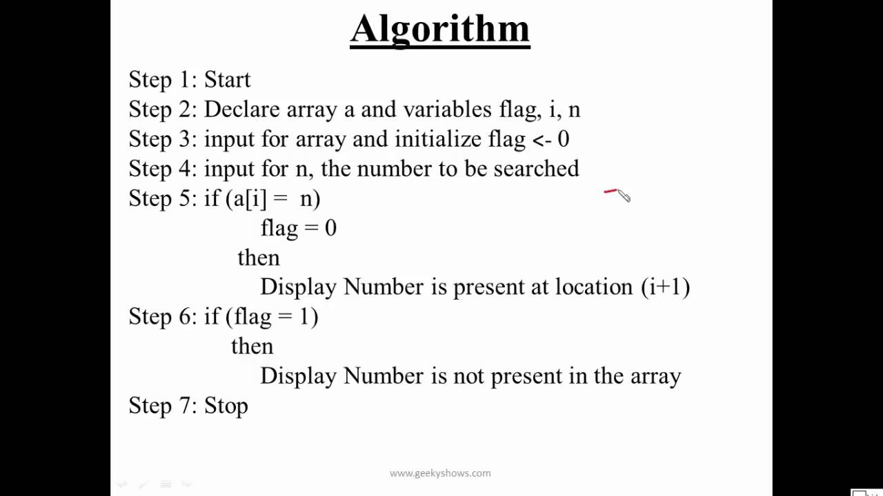
Linear Search
def Linear_Search(A, n)
    for i in range(len(A)):
        if A[i] == n:
            return i
    return -1
Look at each element in turn and one after another, until the value
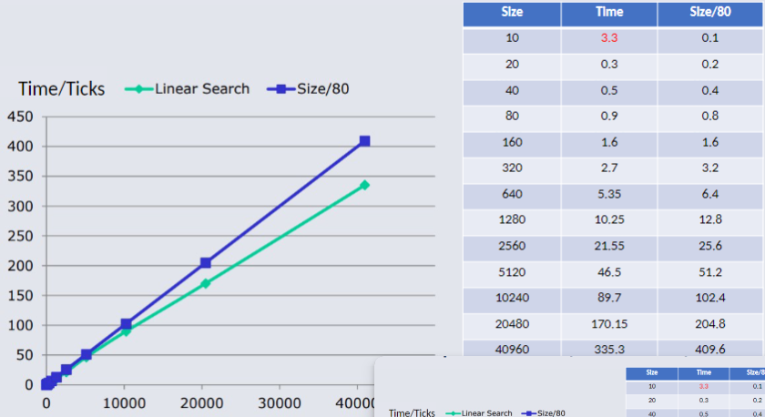
n is found, and then return the index in the array of the location of the wanted value. If the value is not found return -1. Look-Up Time VS Size (Linear Search)
Binary Search
def binary_search(A, x, low, high):
    for i in range(low, high):
    mid = (low, high) / 2
    if (x == A[mid]): return mid
    else if (x > A[mid]): low = mid + 1
    else: return -1

# Example Usage
A = []
The array for Binary Search MUST be sorted. So that the range can be used to hold all items.
While the range is more than one element look at the middle of the range.
Adjust the range to be top or bottom half.
Return the position if you find the target in the only remaining place.
Return -1 if the target is not found.
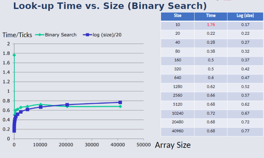
Look-Up Time VS Size (Binary Search)
Conclusion of Experiment
Linear Search:
- Time Proportional to array size (n)
Binary Search:
- Time proportional to log (array size); (log n)
Developing A Model
Selecting an Algorithm
When developing a model, finding an algorithm that can match the key operations intended to be met to meet the expectations of the solution
In regards to the previous experiment, the key operation to be found is; Searching being able to find a target based on a array of elements.
Develop Performance Formula
Developing a formula in relation to the number of times the Key Operation is used in correlation to the array's size.
(n) of the input:
- Linear Search: Number of Comparisons = k * n
- Binary Search: Number of Comparisons = k * log(n)
- Throw away all but the fastest growing term
- Throw away all constant coefficient of this term.
- Linear O(n) Binary O(log(n))
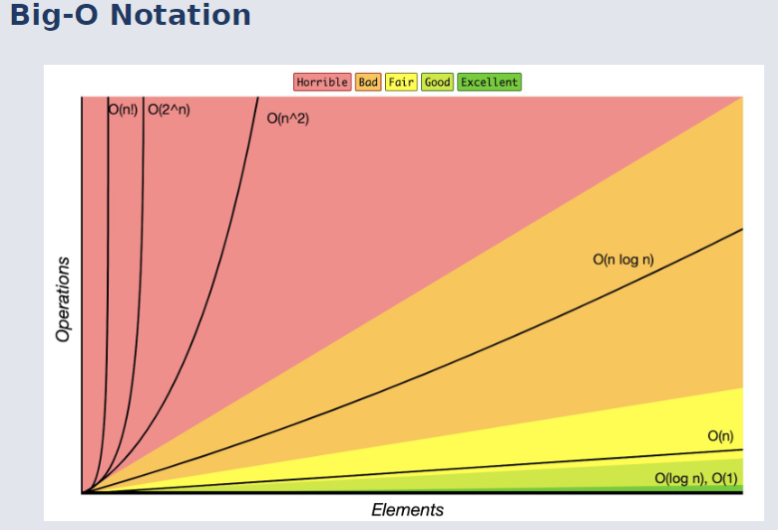
Asymptotic Computational Complexity
Big O, which stands for "in the order of O" is a guide which is not guaranteed to result in the most optimal solution, however, it is considered a useful predictor as an identifier of the performance of an algorithm.
Big-O Notation
Upper Bound
The Upper Bound can be described to be like a ceiling.
While it does not present the length of time, the algorithm will take to run, as this is dependent on other factors such as the size of the input. It instead gives a guarantee that the algorithm will not take longer than the big o value that represents its efficiency.
The upper bound describes the worse-case scenario for an algorithm's resource usage.
Temporal & Spatial
This module only focuses on the temporal aspect of an algorithm.
What is 'n'?
n refers to the input.
i.e. specifically the size of the input:
- the amount of elements in the array
- length of string
Simplification
The formula may be:
n^2+4n+10
n = 1
1^2 + 4 * 1 + 10 = 15
n = 2
2^2 + 4 * 2 + 10 = 22
n = 10
10^2 + 4 * 10 + 10 = 150
n = 1000
1000^2 + 4 * 1000 + 10 = 1004010
As n grows, the n² term (e.g., 1,000,000 for n = 1000) overwhelmingly dominates the lower-order terms (4,000 and 10).
The Maths Bit
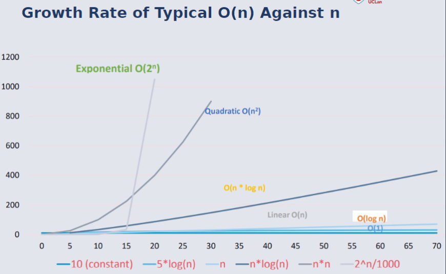
n= Linear Growth (n grows in a straight line like a sequential search)n^2= quadratic growth or n x n operations Often characterised by a nested loop as seen in some sort algorithmsn^2,n^3, etc as above n x n x n but referred to as polynomials.2^nis exponential and therefore every time anothernis added to the number of operations to perform doubles.
Log or Log2
Log(n) or more commonly in computing Log2(n).
The logarithm is simply the number of times a value can be halved.
Logarithm Explain Example
16 / 2 = 8
8 / 2 = 4
4 / 2 = 2
2 / 1 = 1
At which point log2(16) = 4 as 16 can be halved 4 times until it would reach a negative number.
Reverse operations of Log2 should also be noted: Log2(16) = 4 is equal to 2^4=16
Logarithm's make great algorithms because they grow slowly
Growth Rate of Typical O(n) Against n
What is log(n)
| n | n = | log2(n) |
|---|---|---|
| 0 | impossible | impossible |
| 1 | 0 | |
| 2 | 1 | |
| 4 | 2 | |
| 8 | 3 | |
| 16 | 4 | |
| 32 | 5 | |
| 64 | 6 | |
| 128 | 7 | |
| 256 | 8 | |
| 512 | 9 | |
| 1024 | 10 | |
x = log2(n) | ||
n = 2x |
While it is possible to use other bases, 2 is common in computing due to binary only having two usable values.
The table above demonstrates how the key feature of using logarithms with algorithms is that it grows slowly.
Example: BubbleSort
def bubble_sort(A): # Array Input is expected to be sorted.
    n = len(A) # length of array
    swapped = False
for i in range(n - 1): # Range(n) works but will repeat one more time than needed.
    for j in range(0, n - i - 1):
        if (A[j] > A[j + 1]):
            swapped = True
            A[j], A[j + 1] = A[j + 1], A[j]

    if not swapped: # No swaps have occurred.
        return
Number of Comparisons will be:
n * (n - 1) = n^2 - n
Dropping slower terms gives O(n^2).
Lecture 4 - Sort Algorithms