CO2412 Computational Thinking Contents
Lecture 3 - Complexity and Efficiency
Lecture 4 - Sort Algorithms.pdf
An Overview of Sort Algorithms & An Introduction to Optimisations
Sorting Algorithms
Sorting is a common problem in computing. Sorting sequences can be described as follows:
- Input: A sequence of n numbers are provided. i.e. [4,3,2,1,5,6]
- Output: Sorted inputted sequence returned. i.e. [1,2,3,4,5,6]
Bubble Sort Algorithm O(n)
1) function bubble_sort(data_list)
2) n = length of list
3) for start of list to end of list - 1 do as i (current index)
4) for end of list to current index - 1 do as j
5) if data_list[j] < data_list[j - 1] do
6) swap data_list[j] with data_list[j - 1]
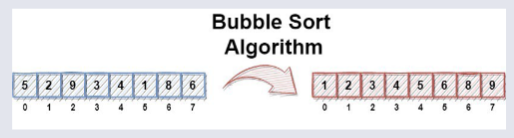
Bubble Sort works by repeatedly swapping the adjacent elements that are in the wrong order.
Insertion Sort Algorithm O(n)
To sort through an array of size n in ascending order.
Insertion Sort Step-By-Step
1) iterate through the second element of the array to the end of the array
2) Compare the current element (The Key) to its previous value
3) If the key (current element) is smaller than the previous element then
4) Move the greater elements one position up to make space for the swapped element
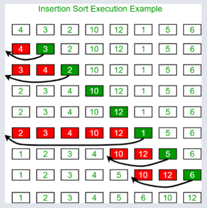
The array is split into a sorted and unsorted part. Values from the unsorted part are picked and placed at the correct position in the sorted part.
Merge Sort Algorithm O(n log n)
Merge sort is another algorithm that can be utilised to sort an array of n size.
Merge-Sort Sort Step-By-Step
- 1) Divide: Recursively split the array into two halves until sub-lists contain single elements.
- 2) Conquer: Merge pairs of sub-lists, sorting them during the merge process.
- 3) Combine: Continue merging until the entire array is sorted.
![[Pasted image 20250426131436.png]]
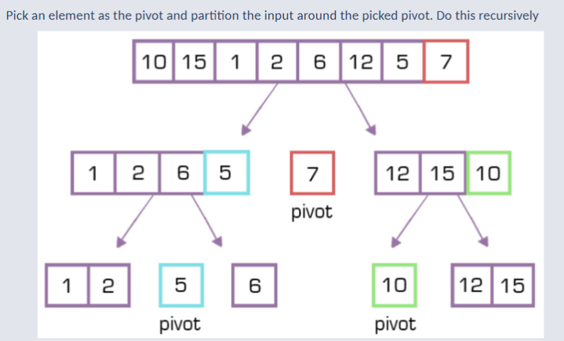
Quick Sort O(n log n)
QuickSort uses partitions around a pivot point and sorts the subarrays in-place.
Different to Merge Sort as it doesn't use memory when creating many sub-arrays.
Quick-Sort Step-By-Step
1) Pick a pivot point such as the last element. (e.g., first element, middle element, random, or median-of-three)
2) Partition the array so that:
- Elements less than or equal to the pivot are placed to its left.
- Elements greater than the pivot are placed to its right.
1) Recursively Apply QuickSort to the Sub-Arrays
def quick_sort(A, low, high):
    if low < high:
        pi = partition(A, low, high)
        quick_sort(A, low, pi - 1)
        quick_sort(A, pi + 1, high)

def partition(A, low, high):
    pivot = A[high]
    i = low - 1
    for j in range(low, high - 1):
        if A[j] <= pivot:
            i = i + 1
            A[i] = A[j]
    A[i + 1] = A[high]
    return i + 1
Optimisation
Problems with Optimisation
For an algorithm to be considered correct it must consistently produce the expected result for every input.
Optimisation aims to find the best solution from a set of possible alternatives.
This range of options is referred to as the search space or solution space.
Typically, these solutions are represented as vectors of variables.
The optimal choice is the one that achieves the highest value for a clearly defined criterion.
Conditions
Alternatives have to be feasible, which is defined as meeting the number of constraints defined in the problem.
Mathematical optimisation appears trivial (easier than sorting) however optimising often requires searching over many permutations of other input objects.
Whilist sorting only requires knowing the ordering of N objects, optimisation focuses on the N! candidates to search and test. i.e. an exponential function of input size.
Optimisation is about how to organise the searching of this set to obtain results efficiently in time and/or space.
An Example - Knapsack 0/1
John delivers packages from a distribution warehouse to a store. Each package has a weight and a value.
John has a small van which can only carry up to a set weight, this is called the capacity. Each time John loads his van at the warehouse he must maximise the value of the items he carries.
To keep things simple we’ll say that the weight of the item is the same as the value and the capacity of John’s van is 10.
John has 4 items to pick
| Item | 1 | 2 | 3 | 4 |
|---|---|---|---|---|
| Weight | 5 | 4 | 3 | 2 |
| Value | 5 | 4 | 3 | 2 |
John decides the best method to maximise the value is to always keep the item with the highest value until he can carry no more, which is known as the greedy approach or the greedy algorithm.
Greedy ALWAYS makes the optimal choice at each step.
John selects item 1 as this has the highest value and puts it in the value, then he selects the next most valuable item; item 2 and puts this in the van.
John is now carrying 2 items with a value and weight of 9.
John tries to put item 3 into the van but cannot as it takes him over the limit so he discards this as well and sets off to the store with the items. In this case being item 1 and item 2.
The Greedy Algorithm is not a guaranteed to produce an optimal solution to the 0/1 knapsack problem presented.
Solution is Enumeration
When John returns to the warehouse he is called to the supervisor's office to explain why he set off without maximising his load.
John's supervisor tells him that if he had selected items; 1,3 and 4 he could of maximised the value of the items he carried.
In future he tells John to try all the combinations of items before setting off to ensure he gets the best possible solution as such a full enumeration or full brute force solution can be undertaken.
As an item can either be taken or left there are:
Amount of Categories (Weight, Value) divided by amount of items (4 Items).
2^4 - 1 (15) possible combinations for John to try.
The complexity is therefore O(2^n) which means enumeration has exponential growth.
Problem with Solution
After several months of successfully John passes his heavy goods vehicle driving test.
Given this vehicle is a much better vehicle with a far bigger capacity and therefore has more items to carry potentially of a higher value.
Typically the new vehicle can carry 20 items at a time. John tries to calculate the combinations but quickly gives up.
Assuming there are 20 items to pick from John now has 2^20 - 1 (n items) to pick from.
This results in a total of 2 (Weight and Value) to the power of 20 (20 possible items) - 1 (Accounting for an empty van, which is not a feasible alternative as John must deliver the maximum amount of items to the warehouse.) = 1,048,575 possible combinations.
Each additional item that is added, increases the number of combinations exponentially.
Enumeration has the worse case run time of O(2^n).
Enumeration - A Summary
Enumeration is conceptually simple:
- Compute all possible combinations and keep the best feasible solution
Why Enumerate?
It is optimal - always get the best solution.
Space Efficienct - only ever need to store the current task.
however:
The solution space grows exponentially. It rapidly becomes unfeasible to compute all solutions.