CO2412 Computational Thinking Contents
Lecture 8 - Graph Theory
Lecture 9 - BFS (Breadth First Search) & DFS (Depth-First Search).pdf
Breadth First Search & Depth First Search
Search Algorithms
During the lectures the following search algorthms have been discussed:
- Linear Search #find-link
- Binary Search
- Binary Search Trees
This lecture will cover:
- Breadth-First Search
- Depth-First Search
Here’s an enhanced version of your explanation with smoother phrasing and clear structure:
Adjacency Matrix
In graph theory, when two vertices are connected by an edge, they are said to be adjacent.
An adjacency matrix is a way to represent adjacency relationships in a graph.
A square matrix is utilised:
- 1 indicates that two vertices are connected by an edge (adjacent).
- 0 indicates that two vertices are not connected.
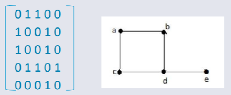
Properties of Adjacency Matrices:
- For graphs with no loops, the diagonal of the matrix will always contain 0s, as no vertex connects to itself.
- In a non-directed graph, the adjacency matrix is symmetrical. This is because edges in an undirected graph can be traversed in either direction, making the relationship mutuals.
Search Space in Algorithms
The Search Space is the set of all possible states or solutions that an algorithm must explore in order to solve a problem.
Key Regions of Search Space:
Explored: These are the regions or states that have already been searched and are already known.
Unexplored: These are states that have not yet been discovered or examined.
Waiting To Explore (Known as Fridge or Frontier): These are states that have been discovered but not yet explored fully.
Breadth-First Search
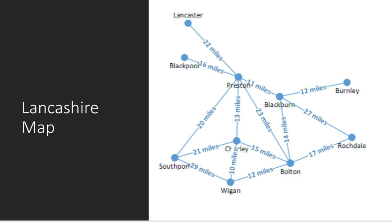
Shortest Path from Blackburn to Southport
BFS takes the shallowest path first.
The BFS algorithm is a function which accepts the inital state and the goal as test arguments.
The states are ordered alphabetically.
Using the FIFO (First-In First-Out) data structure. (Queue to process the Frontier states)
Uses a set to hold the done states.
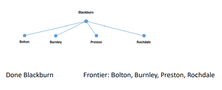
BFS - Blackpool to Southport
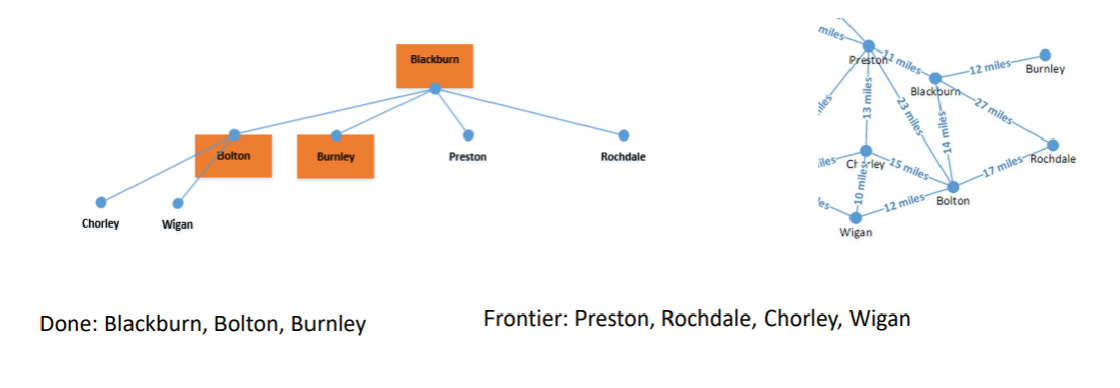
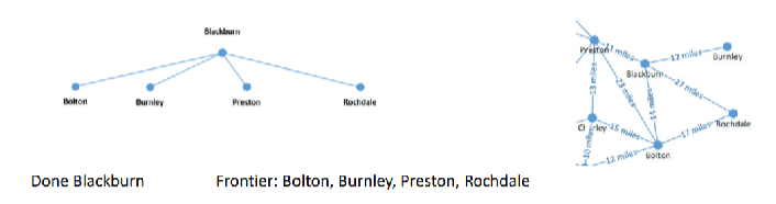
Add the start state Blackburn to the frontier.
Its adjacent vertices (neighbors) are added to the frontier, ensuring breadth-first exploration
As nodes are explored, they are moved to the done states, meaning they won't be revisited.
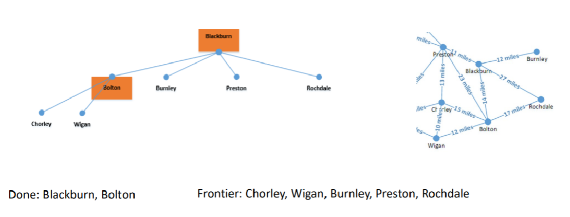
Continuing with Breadth-First Search Bolton was the first into the queue, so that is processed next. Adding Bolton into the done state, since it is not what we are trying to find.
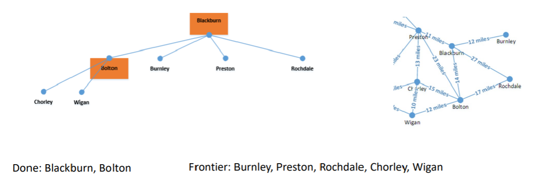
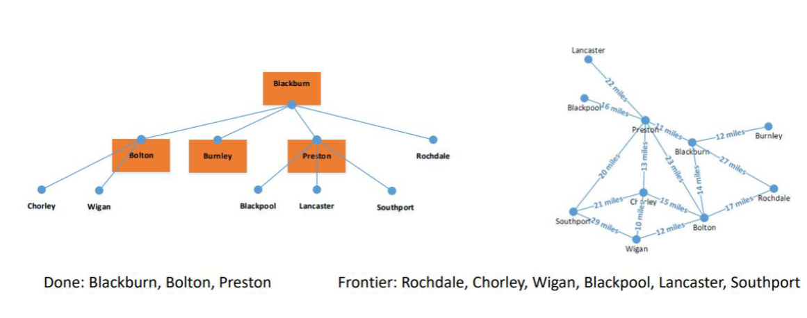
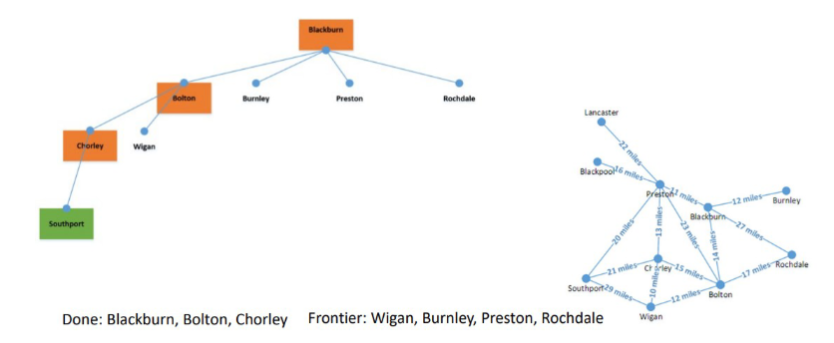
Next Burnley gets added to the done states as it once again isn't the location (Southport) that the BFS is trying to find the shortest path for.
Next onto Preston since Soutport is in Preston, as per the diagram presented, the BFS finds Preston, which gets added to the done states.
However, now Preston's neighbours are added to the Frontier of possible options to the shortest path.
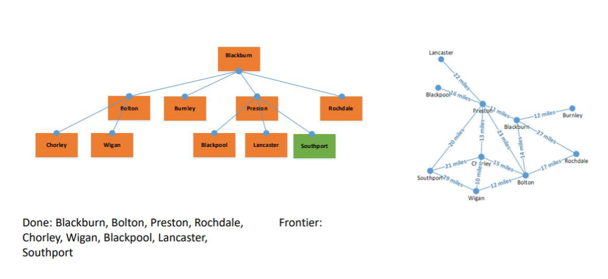
Rochdale is is added to the done states.
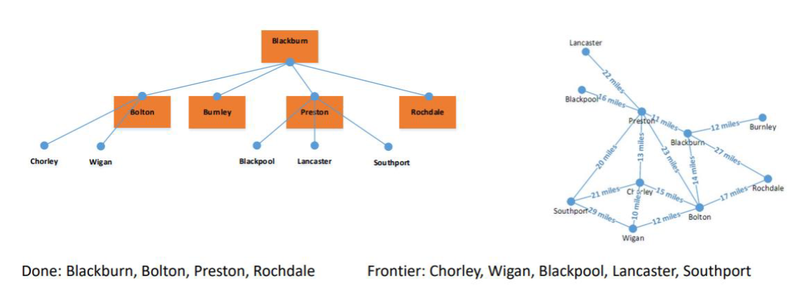
This process is continued until options are entered into the done states.

Breadth-First Search Cost
Optimal: BFS is optimal if the cost of every step is the same (uniform)#
(e.g. 1 Step per edge.)
Complete - Yes, the BFS is garanteed to find a solution is the search space is finite.
Time Complexity: (1 + b + b^2 + b^3 + etc + b^n))
(b) is the branching factor (average number of child nodes per node)
(n) is the depth of the solution
Implementation: BFS uses a FIFO (First In First Out) queue data structure to manage the Frontier.
When to use BFS
Best suited for shallow search spaces.
Can be optimised by caching the previous searches.
BFS Cost Example Table
| Depth | Nodes | Time | Memory (Space) |
|---|---|---|---|
| 2 | 110 | .11 miliseconds | 107 KB |
| 4 | 11,110 | 11 miliseconds | 10.6 MB |
| 6 | 10^6 | 1.1 seconds | 1 GB |
| 8 | 10^8 | 2 minutes | 103 GB |
| 10 | 10^10 | 3 hours | 10 TB |
| 12 | 10^12 | 13 days | 1 PB |
| 14 | 10^14 | 3.5 years | 99 PB |
| 16 | 10^15 | 350 years | 10 Exabytes |
| b = 10.1 million nodes per second. | |||
| 1000 bytes per node. |
Depth-First Search
DFS - Blackburn To Southport
Takes the deepest path first approach.
The algorithm is a function which accepts an inital state and a goal state.
The order of the states will be alphabetical.
Uses a LIFO data structure. (Stack to process Frontier states)
Uses a set to hold the done states.
As with BFS we start by adding "Blackburn" to the Frontier, since this is not what we are looking for. This will be added to the done states.
Its adjacent vertices are then added to the Frontier.
They are pushed onto the Frontier stack in Reverse order.
DFS Cost
Optimal: Not guaranteed, as DFS soes not necessarily find the Shortest Path it may get stuck in deeper branches before finding the solution.
Complete: Yes, if the search space is finite, and there's no infinite depth, DFS is complete.
Time Complexity: O(b^n) where:
(b) is the branching factor (average number of child nodes per node)
(n) is the maximum depth of the search space
Implementation: DFS uses a LIFO Stack to manage the Frontier.
When To Use DFS
Best suited for problems where the solution lies deep in the search space otr when memory is a critical constraint.
A drawback to DFS is that it may explore inefficiently if the solution is far from the initally explored path or in shallower areas.
DFS Space Advantage
Using the BFS Cost Table from earlier.
Recall that:
- b = 10
- 1 million nodes per second
- 1000 bytes per node.
DFS has an advantage in terms of space over BFS.
Space = O(b*n)
Depth = 16
10 x 16 = 160 x 1000 bytes per node = 160,000 bytes.
160,000 / 1024 = (approx) 156 KB
DFS = 156KB
BFS = 10 Exabytes